Beamformed
Brief
Format
Dynamic spectrum raw data is stored in the form of HDF5 file, which is a type of self described file.
The metadata is in the header of the HDF5 file, and the data is stored in the body of the file.
Here is a general exampel of how to retrive the information from header and plot the dynamic spectrum with h5py.
Tutorial .h5
Size
Raw data is always huge, a typical observation of 2 hours, saved in hdf5 file as float32,
time resolution 1/96 second, 4096 frequency channels, the data size of one beam single polarization is:
\(\rm 4[Byte] \cdot 7200[s] \cdot 96 \cdot 4096[ch] =10.54 GB\).
To form a tied array beam (TAB) imaging, there will be 127 beams, with 4 polarizations, the total size of 2 hours of TAB observation is: 5.3 TB.
Calibration
The dynamic spectrum download from Long-time-archive (LTA) is not calibrated, the observation is usualy performed with a calibrator observation, we can have gaincal calibration for the dynamic spectrum by doing the following steps:
Download the target and calibrator observation from LTA
Apply averaging on the calibrator observation to get a instrument reponse of the calibrator (\(I_c(\nu)\))
Calculate the gain with the \(\rm{gain} =\it \frac{M_c(\nu)}{I_c(\nu)}\),where \(M_c\) is the model of the flux of the target object (e.g. CasA, VirA…).
Apply the gain to the target (Sun) dynamic spectrum with \({I_t} = {I}_{t0} \times \rm{gain}\)
With this method, we can have a roughly calibrated dynamic spectrum, while the beam pointing is not considered in this procedure, the errorbar could be very large.
Quick View
To cope with the large data size, providing some quick access to the dynamic spectrum, we can downsample the data to a smaller dimension.
FitsCube
This is a demo to show how to use FitsCube to read the data and produce the TAB image. Demo
Quick View of the LOFAR beamform:
Go to a empty directory, run the following command.
git clone https://github.com/peijin94/LOFAR-Sun-tools.git
cd LOFAR-Sun-tools
# (conda activate xxx)
python setup.py install
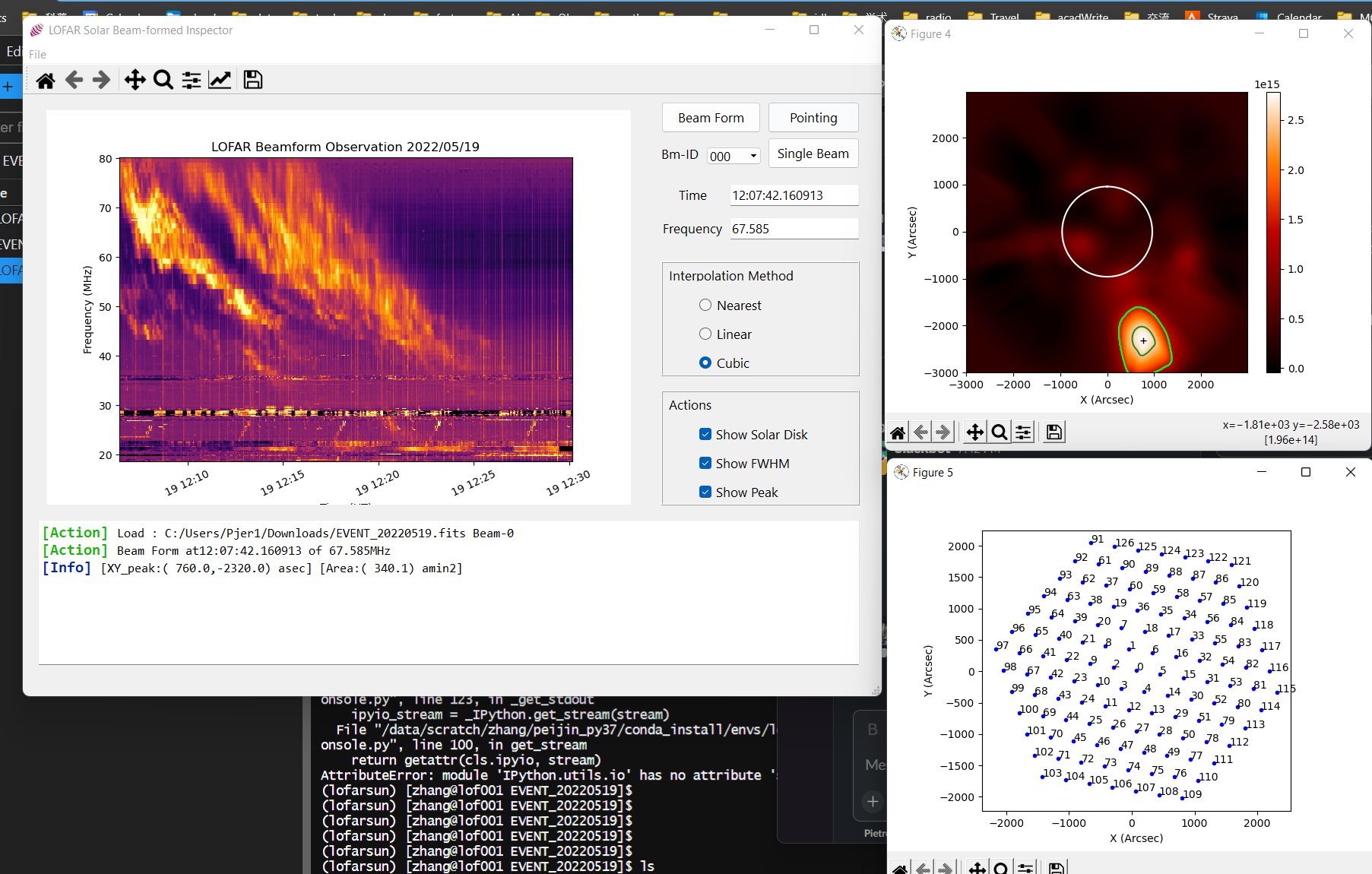
Run quick view for TAB-cube-fits:
# (conda activate xxx)
lofarBFcube
Then load beamformed imaging fits and preview: